Public Data Access Overview / Synthetic Absorption Line Spectral Almanac (SALSA)
This page provides access to the Synthetic Absorption Line Spectral Almanac (SALSA), as described in Nelson et al. (2025).
Here is a random example of one of the many millions of absorption spectra available (refresh to see another):
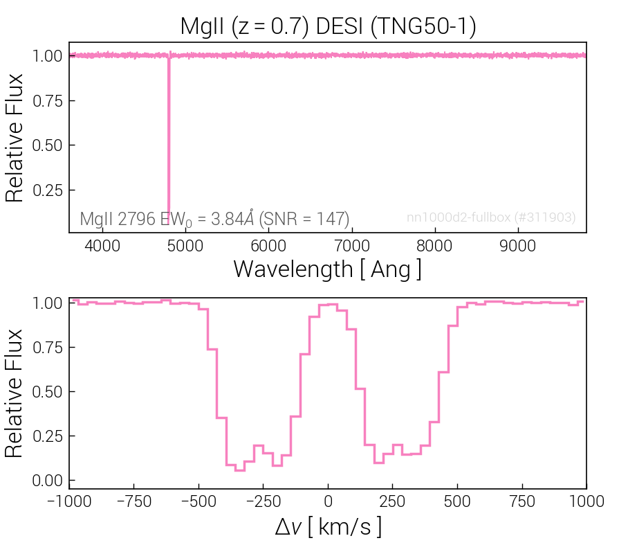
We are creating mock, or "synthetic", absorption spectra by drawing lines-of-sight through cosmological hydrodynamical simulations. This dataset spans a diverse range of ions, transitions, instruments, observational characteristics, modeling assumptions, redshifts, and so on. It is also not limited to one simulation, but includes spectra created from various publicly available cosmological simulations.
The image below shows a schematic overview of the setup: a sightline traverses a simulated volume (dashed white line) and (potentially) intersects the projected virial radius (white circle) of a galaxy, as shown in the lower-right inset. The circumgalactic medium of this halo shows a complex and multi-scale morphology, including bubble-like features driven by galactic feedback. The resulting density and kinematic structure is imprinted in observable spectroscopic signatures such as the NeVIII 780, 770 doublet (mock COS/G130M; orange) and CIV 1548, 1550 doublet (mock KECK/HIRES, at z=2; blue).

Available Spectra
The currently available spectra are shown, and can be downloaded, in the following table. Select simulation:
Instrument legend: 4MOST-HRS COS-G130M COS-G160M COS-G185M DESI KECK-HIRES-B14 SDSS-BOSS XSHOOTER-NIR-04 idealized
Sightline legend: n1000d2-fullbox n2000d2-rndfullbox n100d2-rndzoomhalos
Note: the icon [] denotes 'not yet available'. Click to request for the future. The concept of this project is that the number and scope of available spectra is not fixed, but can grow and evolve over time through requests and inputs from interested researchers and the community.
Please get in touch with the details, and we will create and add new spectra.
There are currently [305,000,000] spectra, across [270] files, available.
Data Structure
One spectra file exists for a given combination of: (1) simulation, (2) snapshot, (3) sightline configuration, (4) instrument configuration, (5) ion. All considered transitions of this ion are included.
In each file, they following datasets are present:
wave- 1D dataset with shape (N_wave) giving the wavelength grid in (observed-frame) Angstrom.EW_{line}- 1D datasets with shape (N_spec) of the total equivalent width for each{line}.N_{line}- 1D datasets with shape (N_spec) of the total column density of the (lower transition state) species for each{line}. (Available in some spectra).
Note: based on entire spectrum, not localized to a single absorber. Interpret with caution if more than one absorber present along a sightline.v90_{line}- 1D datasets with shape (N_spec) of the velocity range enclosing 90% of the total flux for each{line}. (Available in some spectra).
Note: based on entire spectrum, not localized to a single absorber. Interpret with caution if more than one absorber present along a sightline.tau_{line}- 2D datasets with shape (N_spec, N_wave) giving the optical depth spectra for each{line}.flux- all transitions are combined to form a 2D dataset with shape (N_spec, N_wave) of the flux spectra, i.e. continuum normalized absorption spectra.
Note: use with caution for ions that include absorption out of non-ground state levels. These transitions have optical depth arrays that assume the respective ground states are fully populated, and this is e.g. incorrect for fine-structure transitions in low-density gas.
flux spectra are just for convenience, and can be reconstructed by summing together the optical depths of all transitions and then computing $f = \exp{(-\tau)}$. For example, for a configuration of $2000^2 = 4$ million spectra for SDSS/BOSS, with 4678 wavelength bins, the optical depth and flux datasets have shapes of $[4000000, 4678]$.
Each file also contains the following metadata:
lineNames- the list of lines i.e. transitions of this ion that are available.ray_dir- unit vector indicating sightline direction, constant for all sightlines.ray_pos- the starting sightline positions, in simulation box coordinates.ray_total_dl- the sightline length, in simulation box units, constant for all sightlines.instrument,redshift,simName, andsnapshot- for reference.
These spectra files are accompanied by sightline files that specify exactly which gas is intersected by each line of sight. In particular, the ordered list of gas intersections -- their global snapshot indices, and intersected path-lengths. This information allows each spectrum to be associated with the individual gas parcels, and thus the physical gas properties, giving rise to the absorption. For convenience, these are split into 16 files per simulation snapshot. Each file contains:
ray_pos- the starting sightline positions, in simulation box coordinates.rays_dl- the pathlengths of the intersected ags cells, in simulation box units.rays_inds- the indices of the intersected gas cells. These index thecell_indsdataset.rays_len- the number of intersections, for each sightline.rays_off- the first entry inrays_indsof this sightline, i.e. the index (or "offset") of this sightline.cell_inds- list of global snapshot gas cell indices that are intersected by all the sightlines in this file.
The structure of these datasets follows the usual offset/length approach, such that the (ordered) list of intersected path-lengths of sightline j are given by rays_dl[rays_off[j]:rays_off[j]+rays_len[j]]. The (ordered) list of intersected gas indices of sightline j are similarly given by inds_j = rays_inds[rays_off[j]:rays_off[j]+rays_len[j]], and the corresponding global simulation snapshot (PartType0) indices are given by cell_inds[inds_j]. A Jupyter notebook is available in the Lab (see below) with examples.
In addition, the original galaxy and halo catalogs of the cosmological simulation at each redshift allow absorption features to be correlated with the properties of intervening galaxies and halos.
Data Access - API
Spectra
The list of all available spectra available for a particular simulation is available at:
In addition to downloading the full spectra files (that can be large, ~GB to ~10s of GB), functionality has been added to the API to ease their use. In particular, an entire spectra file is downloaded (from the table above) via a path such as:
You can download a single spectrum from this file, selecting by its index, by appending ?index=N to the URL, for example:
You can then also change the file format of the request, from .hdf5 to either .json, .csv or .txt, for example:
You can also request a quick plot of this specific spectrum, with a file format of .pdf, .png or .jpg, for example:
You can use ?index=random to randomly select a spectrum from a file, for quick inspection.
To use any of these endpoints, either in your browser or in e.g. a Python script, you can right click on any icon in the table above, select 'Copy Link', and modify it as appropriate.
Sightlines
The list of the corresponding sightline files are available at:
For each snapshot (and configuration), these are split into 16 equally-sized chunks, for convenience. For example, the n1000* configurations, with $1000^2$ total sightlines, have 62,500 sightlines per file. As a result, the spectrum with index 0 is therefore the first sightline from chunk 0, while the spectrum with index 125001 is the second sightline from chunk 2, and so on.
For convenience, the information for one particular sightline with global index N is available from the API by via the path:
i.e. by omitting a particular chunk number, and instead appending ?index=N to the URL. Note that this extraction is slow (several seconds per sightline), so if you are analyzing more than a handful of sightlines, it will be more efficient to download/load the full sightline files directly.
Data Access - JupyterLab
All files are directly available in the online Lab, under the postprocessing/AbsorptionSpectra/ folder of a particular simulation.
In examples/salsa_spectra.ipynb you will find a Jupyter notebook with examples of (i) how spectra can be loaded and visualized, (ii) how to use the group catalogs to connect spectra to nearby galaxies, and (iii) how to use the sightline files to obtain information about the underlying gas causing the absorption.